Building a 3D solar system that actually looks like space
I built 3dsolarsystem.online, here's how I did it and made it look so good.

I spent two days looking at a Mars that was too red. The fix was a missing 1/(16π) in the Rayleigh phase function, a single denominator I’d quietly dropped while porting from a paper. Real-time 3D space rendering is mostly stuff like that, a hundred small physics-correct decisions stacking up, each one worth maybe a percent of perceived realism if you get it right, costing you the same if you skip it.
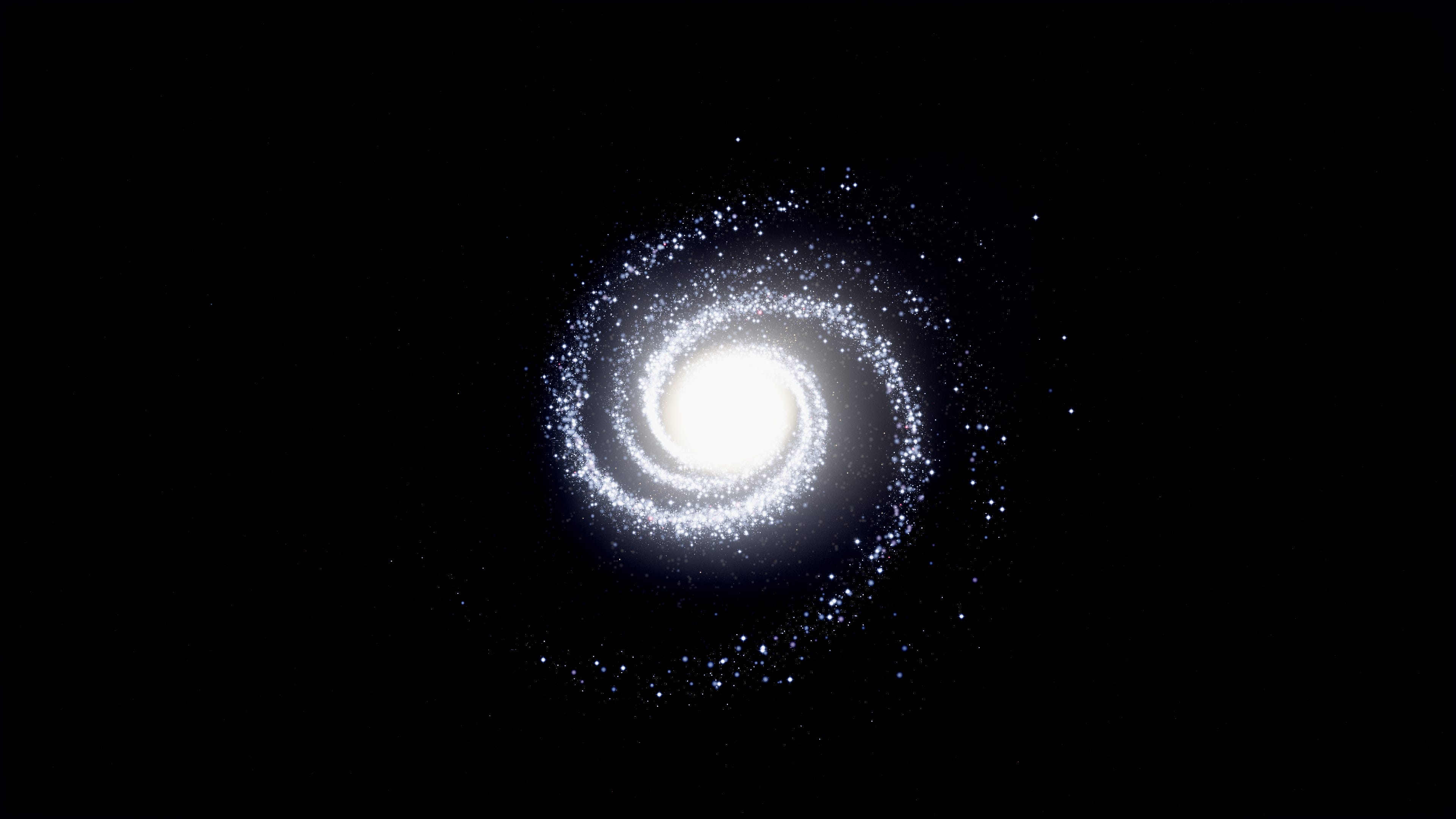
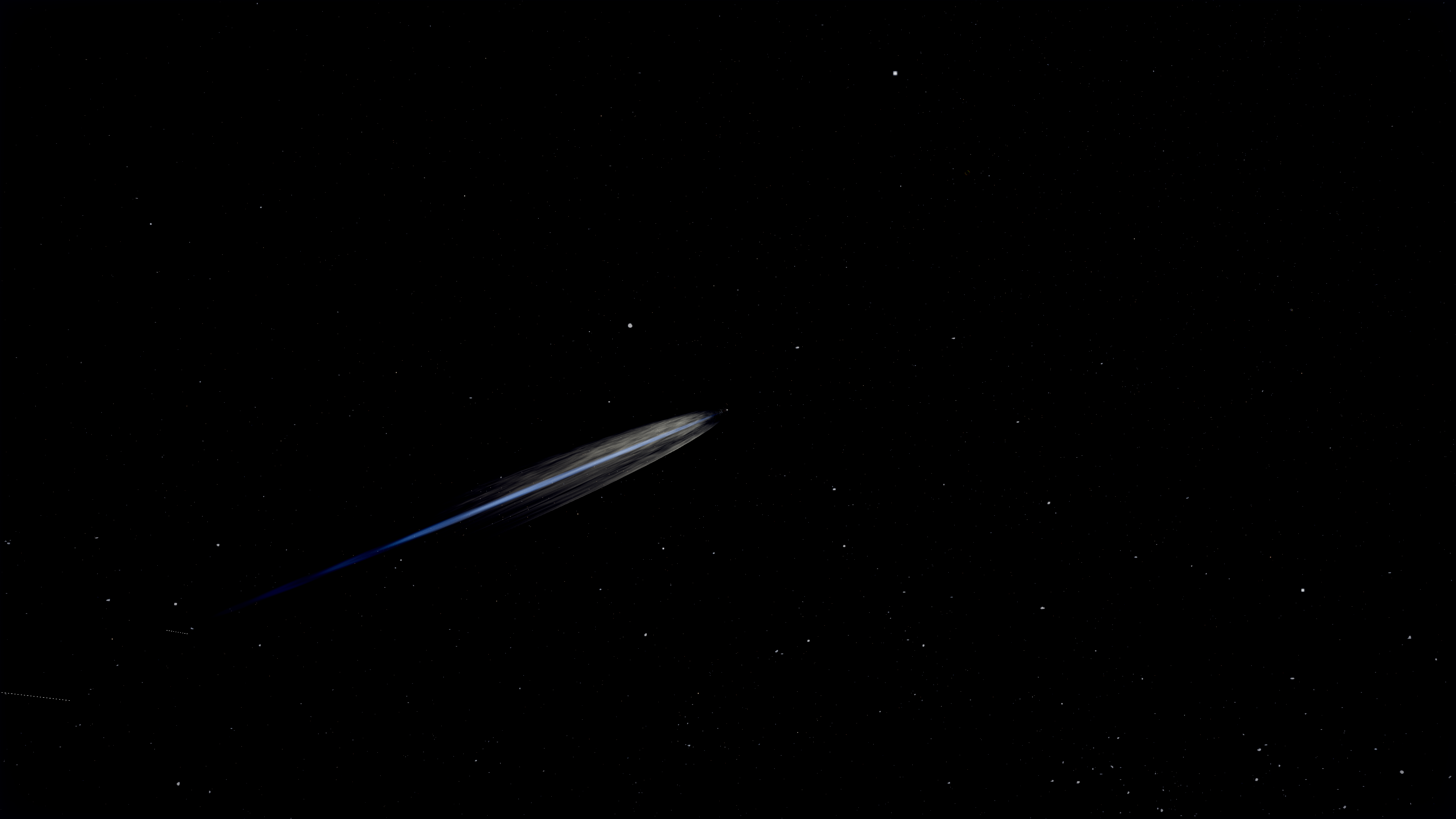
Most browser-based 3D solar systems look like marketing renders. Big bright planets on velvet black, generic glow, planet textures that read as cartoons. I wanted something closer to Cassini and Voyager imagery, real photographic feel with the kind of fidelity that makes you stop scrolling. The result is 3dsolarsystem.online, an interactive 3D viewer of the whole solar system that runs in your browser. Every planet, the major moons, the asteroid belt with proper Kirkwood gaps, comets with ion and dust tails, deep sky objects, the Milky Way disc as a procedural particle system, and a stellar-mass black hole somewhere out past Pluto. You can fly through all of it, switch between a UFO saucer and the Enterprise NCC-1701-D, hit autopilot to anywhere, take photos with cinematic post processing. Free, no signup, just space.
This writeup is about the engineering behind making it actually look like space.
Why realistic space is hard in WebGL
Three things stack against you. Scale, color, shaders, each one bites differently.
Scale first. The solar system is mostly empty space. Earth is a tiny dot at 1 AU, Pluto’s a smaller dot 40 AU out, the sun is a thousand Earth diameters across. You can’t render that 1:1 in a webGL viewport without either a logarithmic depth buffer (which silently breaks every custom shader you have because they don’t ship with the logdepthbuf_* chunks injected by default), or some kind of context-aware near plane management. I went with the latter, a dynamic near plane that shrinks as the camera approaches a body, plus a body-specific safety bubble that lets you fly into Earth’s atmosphere without the depth buffer collapsing into z-fighting on the surface.
Then color. Real space is high dynamic range. Stars are tiny pinpricks brighter than the rest of the scene by orders of magnitude, the sun is a hot pixel pile, planet shadows are essentially black except for ambient cross-illumination from nearby bodies. WebGL gives you an 8-bit sRGB framebuffer by default. Tone mapping is the bridge, ACES Filmic is the right tool, but if your ambient light is too high or your color math is in the wrong color space, the whole scene reads like a poster. Most space demos crush their darks because they don’t tune the ambient, and most of them look yellowed because they’re mixing colors in sRGB instead of OKLCh.
Then shaders. You can’t get realistic atmospheres or gravitational lensing out of MeshStandardMaterial. Almost every interesting body in this project has its own custom GLSL fragment shader, sometimes a custom vertex shader too, all purpose-built for that specific body. The sun, every atmosphere-bearing planet, Saturn’s rings, the gas giant cloud bands, the aurora, the black hole, the wormhole, every one of them. Let me walk through how each piece works.
Starting with the sun
The sun shader is the anchor of the scene. It’s the only emissive body, it lights everything else, and it has to read as plasma rather than orange jello.
The base is a custom fragment shader with multi-octave Fractal Brownian Motion noise driving the surface color. Three layers: ultra-fine for facula sparkle, fine for granulation cells, medium for the larger convection patterns. The fine octave runs at 35x the sphere UV scale, so at close zoom you can count individual granules. At orbital distance the fine layer averages out and you see the broader cell structure.
Color comes from black body radiation curves. Real sun surface temperature is around 5778 Kelvin, which on a Planck curve maps to a warm white slightly biased toward yellow. The rendered color blends from a deep orange in cool intergranular lanes, through warm yellow, up to near-white at the brightest granule cores. I interpolate this in OKLCh space because perceptual interpolation through the chroma arc keeps the colors saturated through the gradient. The same blend in sRGB muddies through grey at the midpoint, which is exactly the visual signature of a stylized render.
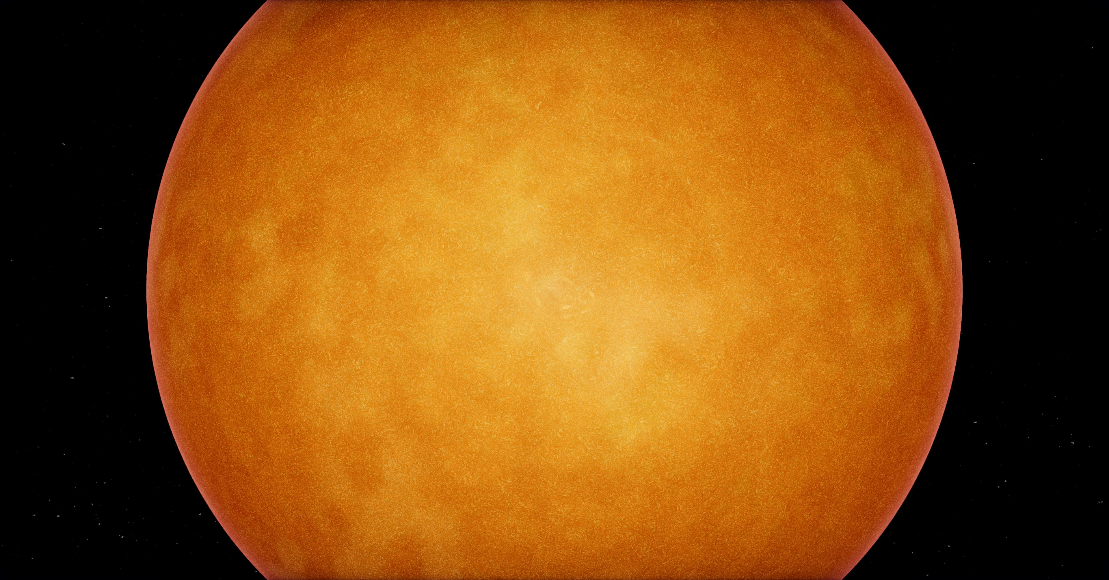
Limb darkening is a simple dot product against the surface normal, raised to a power that matches the empirical solar limb darkening law. The edge of the disc reads a bit darker than the center, which is what gives the sun that “ball of plasma” feel rather than “flat disc with texture”.
Solar prominences are a separate quad facing the camera with their own shader, layered on top of the sun mesh. They animate slowly with low-frequency Perlin noise and only fire at the limb, where they’d actually be visible against the dark background.
The full sun rendering also includes a 6-point diffraction starburst, which is what real cameras do when they point at a bright point source. Screen-space, only triggers when the sun is bright enough on screen. Makes the sun feel like you’re photographing it through a real lens.
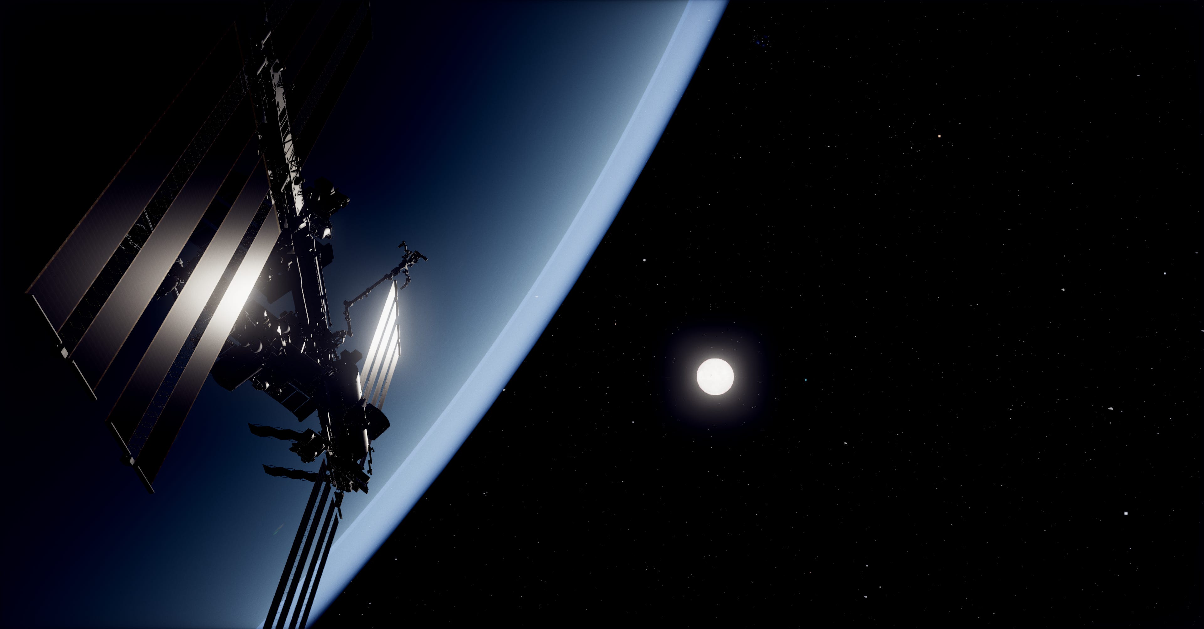
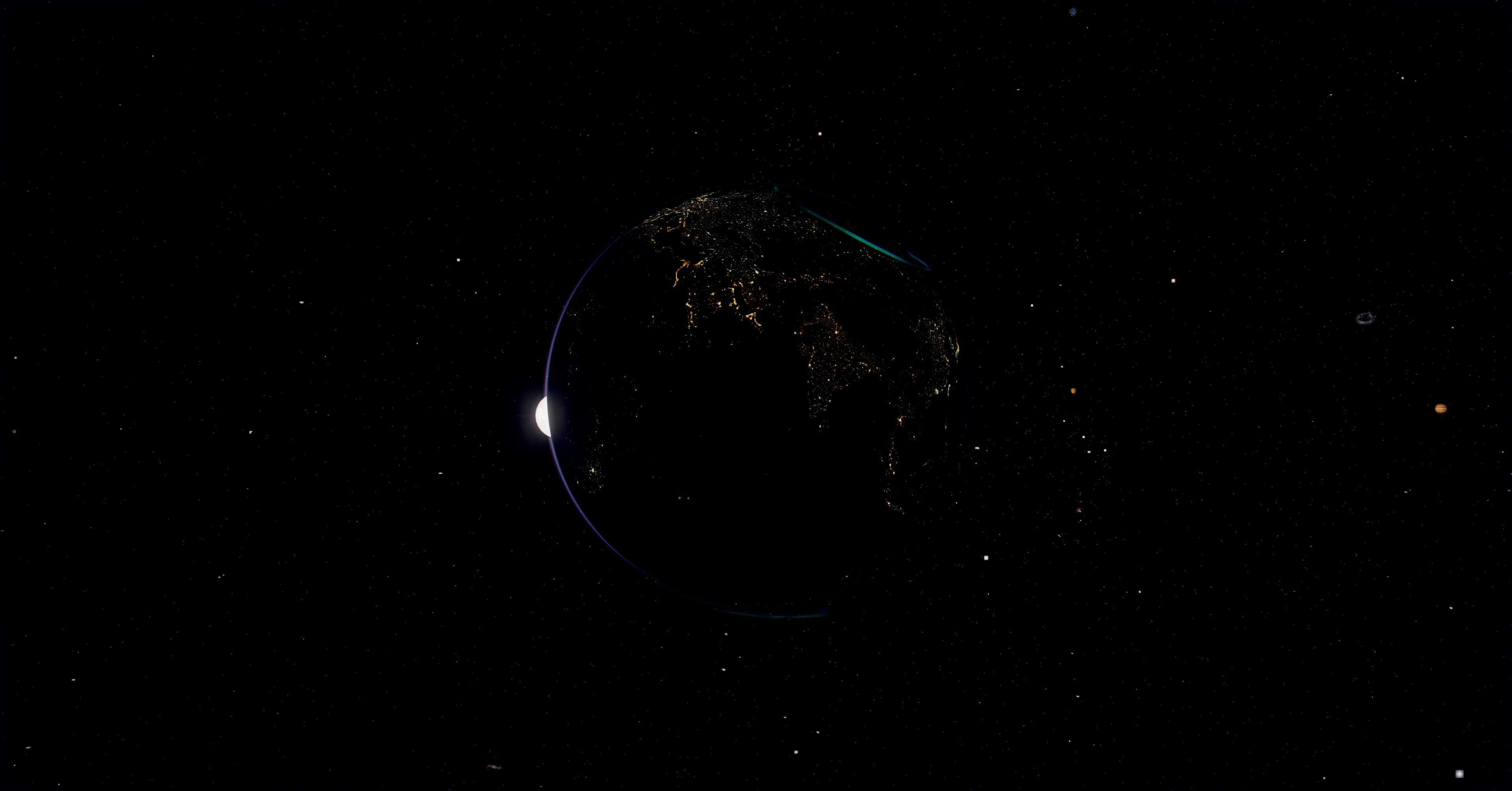
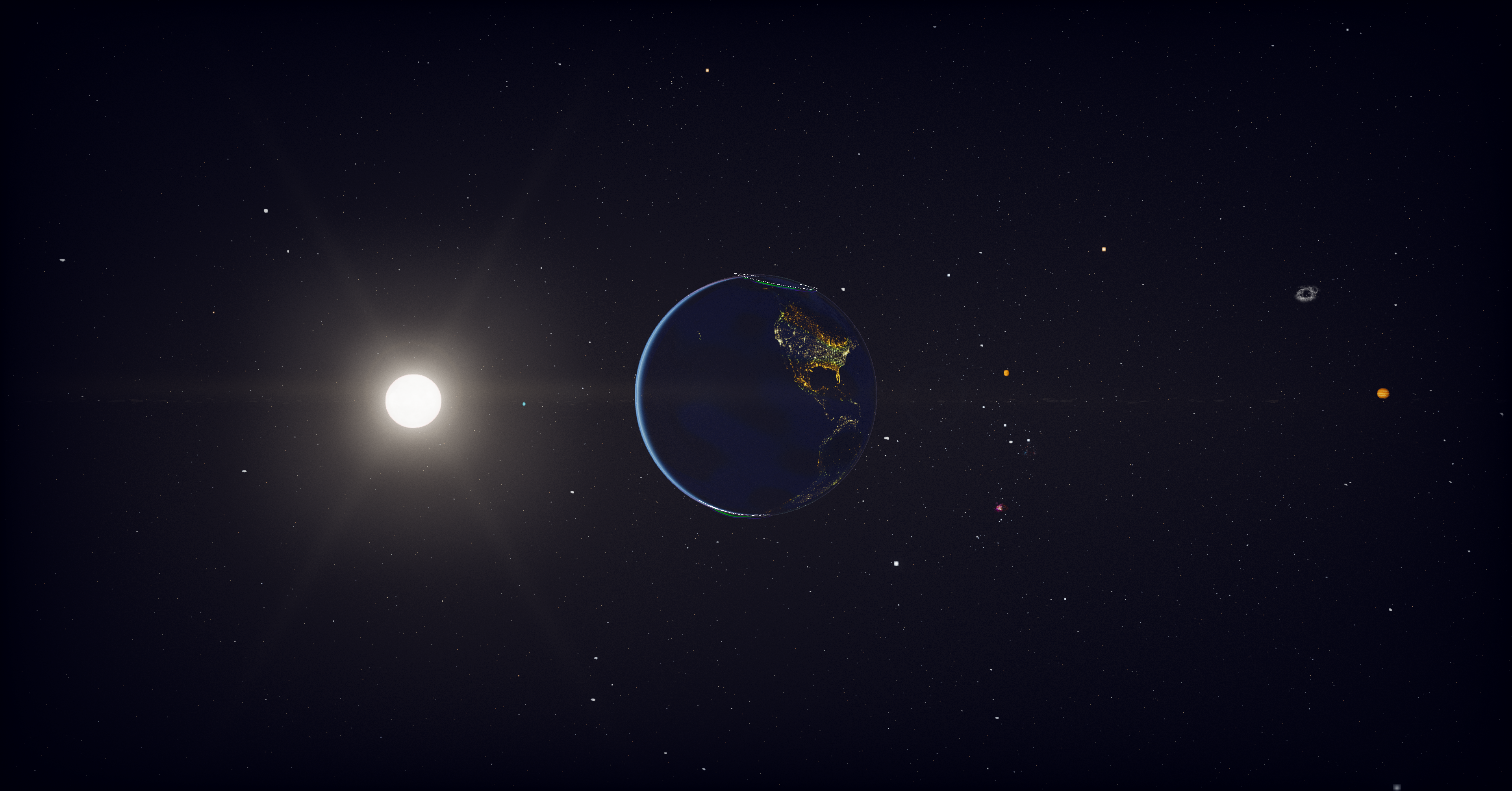
Earth was the hardest planet
Earth has more shader work than every other body combined. One fragment program runs every frame and handles day texture, night-side city lights, terminator warm fade, normal-mapped terrain shading, cloud layer with longitudinal drift, cloud shadows on the surface, ocean specular glint via GGX, snow-and-ice highlight specular, and aerial perspective haze near the limb.
The hard part was aerial perspective. Real Earth from low orbit has a faint cyan-blue haze near the limb, and the planet itself reads as washed out by the atmosphere above it. I added an additive cyan-blue contribution scaled by pow(1 - dot(view, normal), 2.5), small at the center of the disc and large at the limb, multiplied by dayFactor so it doesn’t show up on the night side.
The aurora is a separate shader that wraps the surface mesh and only renders where the magnetic field intersects the polar ovals. Real aurora ovals aren’t circular, they’re deformed by the solar wind, so I use a magnetic field model derived from IGRF coefficients to bend the oval shape. Multiple curtains at different altitudes, each with their own slow drift, so the aurora actually moves and breathes rather than strobing.
Continental elevation comes from a GEBCO bump map. I displace the actual vertices outward by the bump value, scaled to be visible only at the silhouette. Real Earth peaks are 8.85 km against a 6371 km radius, about 0.14% of the radius. I run it at 0.012 in scene units, about 3x exaggerated, just enough that mountain ranges show up at the limb when you fly close.
The atmosphere is its own shader
Every planet that has an atmosphere gets a separate transparent shell, rendered as a BackSide SphereGeometry at radius * atmosphereScale (1.025 for Earth, 1.05 for Venus, and so on). The shell uses additive blending so the atmosphere is light over the planet, not opaque over it.
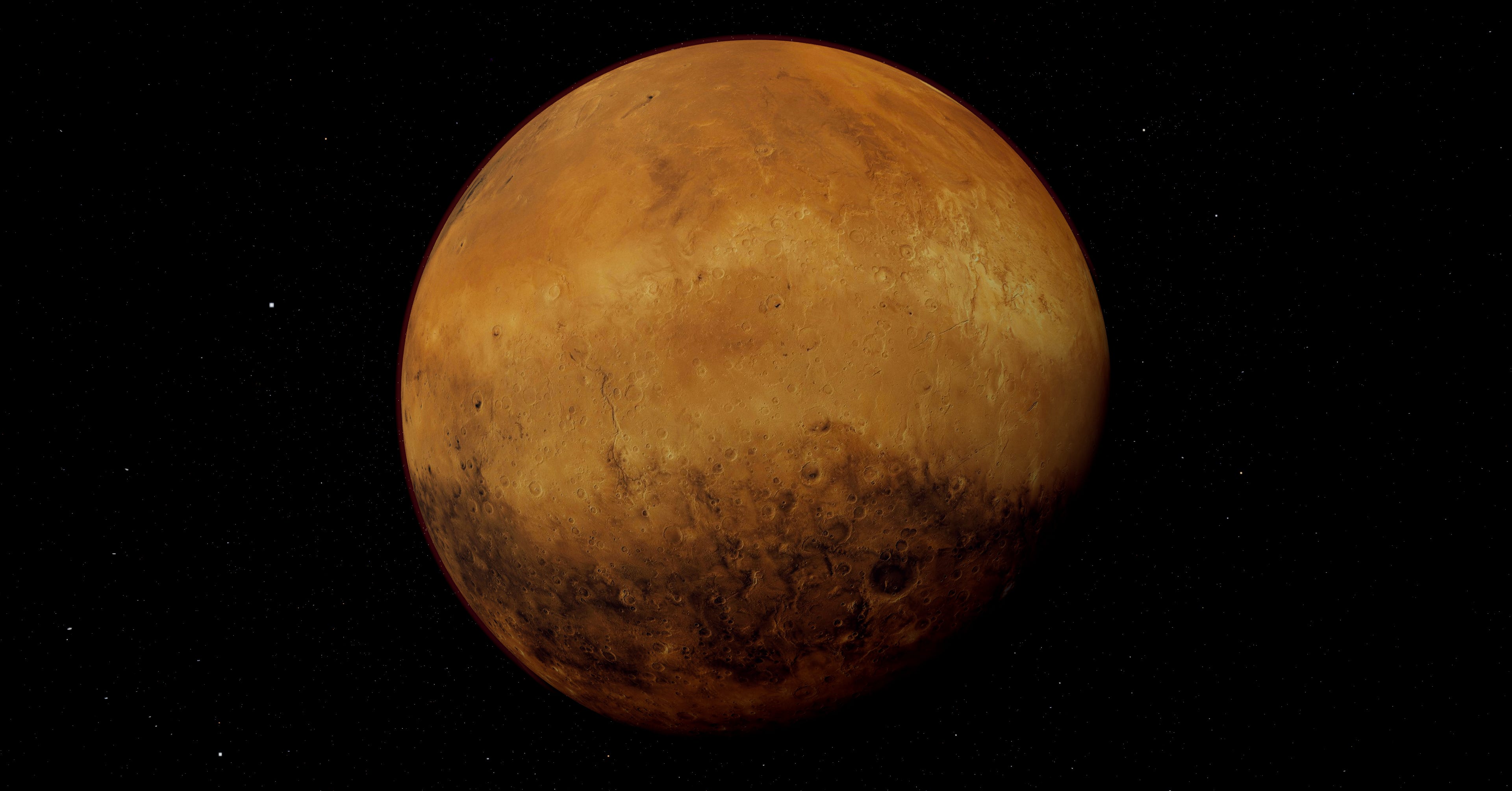
The shader is loosely based on Hillaire 2020’s atmospheric scattering model. Per-fragment, it computes the chord length through the atmosphere shell, applies Rayleigh scattering with proper wavelength-dependent coefficients (5.5e-6, 13e-6, 22.4e-6 for R, G, B), applies the Cornette-Shanks Mie phase function for forward scattering near the sun, and applies ozone extinction in a layer that absorbs the wrong wavelengths.
The Rayleigh phase function uses proper 1/(16π) normalization. This was the Mars-too-red bug from the opening. Without correct normalization the phase function over-contributes blue, which on a Rayleigh-light atmosphere like Mars’s reads as a wrong-colored disc. The Mie phase function I tried in three forms before settling on Cornette-Shanks, which has a tighter sun halo than Henyey-Greenstein and less side-scatter bleed.
Sun-path transmittance is what makes terminators look right. For each fragment, you cast a ray toward the sun and integrate optical depth along that path. The result is the color of the sunlight reaching that fragment, after the atmosphere absorbed the wrong wavelengths on the way in. That’s what gives you the orange-red sunset gradient at the terminator instead of just a dim band. Real photos look that way because the atmospheric chord length to the sun is much longer near the horizon than at the zenith, and Rayleigh scattering removes blue light proportionally to chord length.
Moon eclipse factor was a later addition. When a moon transits between the sun and a planet, the moon’s shadow falls on both the planet surface and the atmosphere. I share the same shadow uniforms between the surface material and the atmosphere material, so they update in lockstep and the eclipse darkening reads as one coherent shadow at the limb.
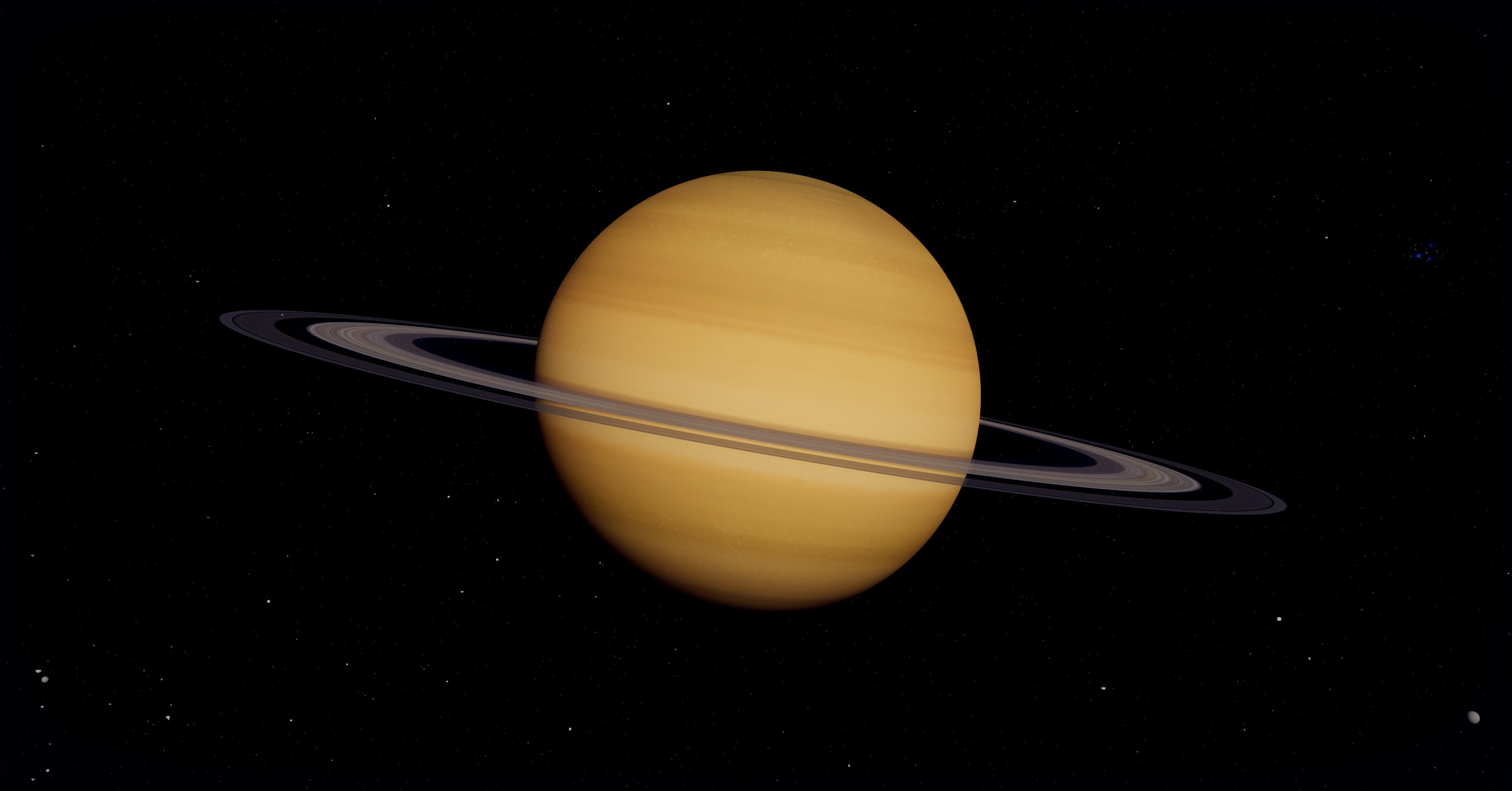
Saturn’s rings deserve special attention
Saturn is iconic, the rings are what make it iconic, so I spent disproportionate time on them.
The rings are a flat disc with a custom shader. The texture comes from a Cassini-derived ring image with two key modifications baked into the GLSL.
The Cassini Division and Encke Gap get explicit alpha drops in the shader. The Cassini Division is the big gap at UV around 0.71 to 0.77, the Encke Gap is the thin one at 0.94. Both are visible from Earth and recognizable in any decent Saturn render, so they need to be there even if the source texture undersells them.
Backlit rings are the second modification. When the camera is on the unlit side, with the sun on the opposite face of the rings, the rings should glow brighter than when lit from the front, because the thin C ring and Cassini Division let light pass through. This is what gives the Cassini “In Saturn’s Shadow” image its iconic look. I implemented it by detecting the camera-to-sun-vs-ring-normal angle and rescaling the alpha so optically-thin regions read brighter when backlit.
Ring spokes are subtle radial dark streaks Voyager and Cassini imaged repeatedly. They’re rare and the cause isn’t fully understood, something about charged ring particles interacting with the magnetic field, but they’re real and worth including. I generate them procedurally with a radial noise field that animates slowly.
Ring shadow projection onto the planet is its own thing. The rings cast a shadow on Saturn’s cloud tops, and that shadow changes shape based on the sun’s angle relative to the ring plane. I implemented it as a ray-march from each Saturn surface fragment toward the sun, testing if the ray passes through the ring disc, then attenuating based on the ring’s optical depth at that radius. Costs about 1% of GPU time and is one of those details nobody consciously notices but the scene feels wrong without.
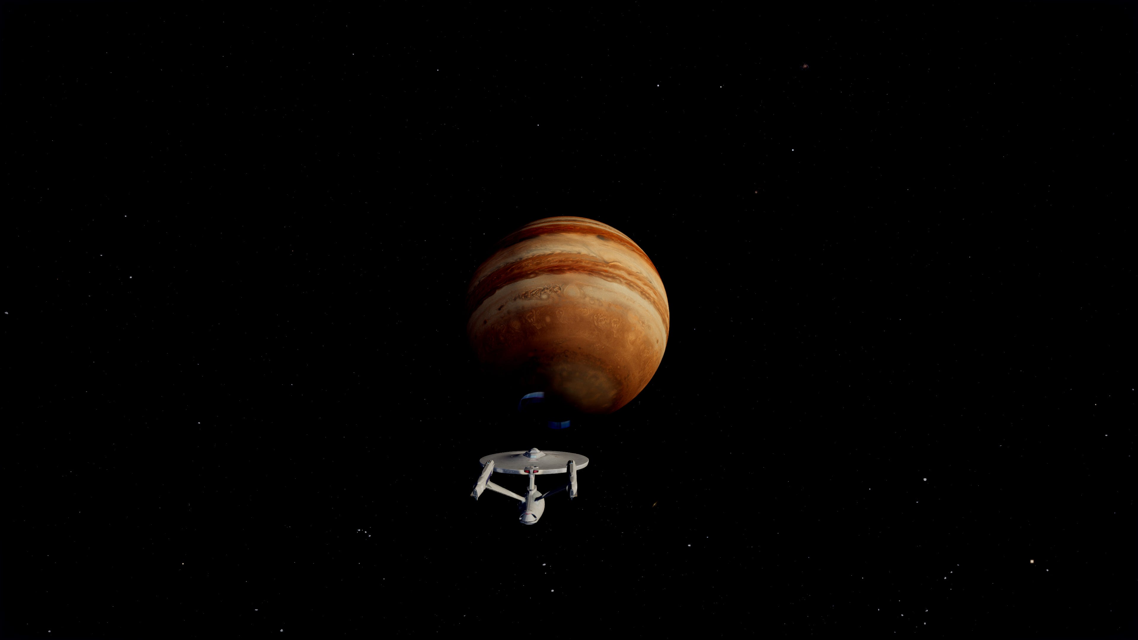
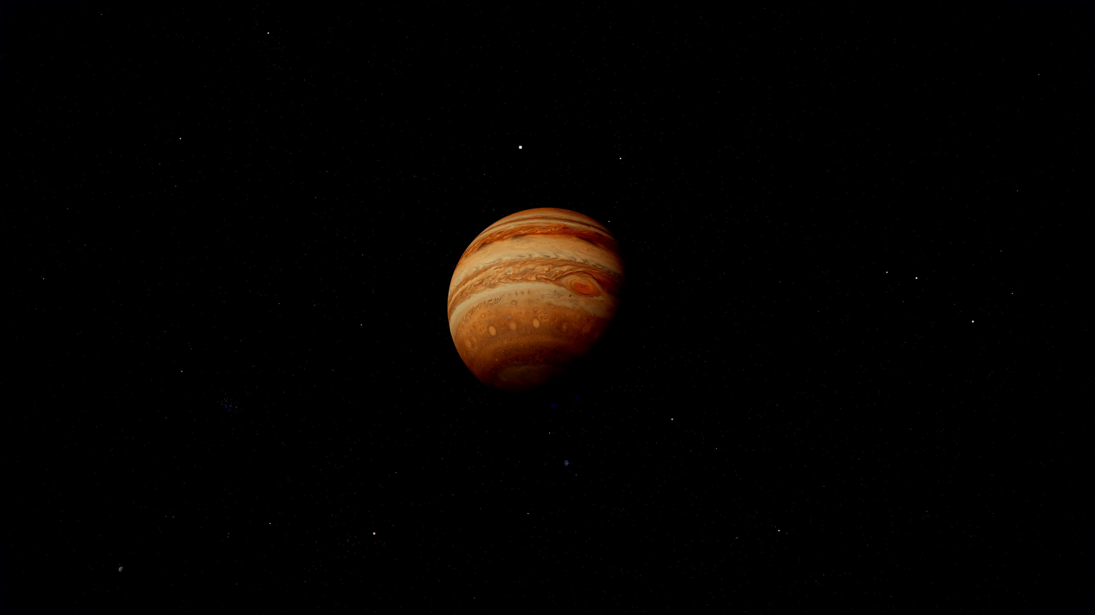
Gas giants need to feel alive
A static texture on a sphere doesn’t sell Jupiter. Real Jupiter has differential rotation (equator faster than poles), the Great Red Spot moves and oscillates, the cloud bands have internal structure.
Differential rotation is a UV shift that scales with cosine of latitude, faster at the equator, slower at the poles, with a small seam-blend at the meridian so the texture wrap doesn’t show. I keep it disabled on Saturn because Saturn’s slower rotation made the seam visible at certain zooms.
The Great Red Spot is a procedural overlay anchored in pre-shift UV space, so it tracks the differential rotation drift. It has a gentle breathing pulse, about 30 seconds period, that matches the slow size oscillation the real GRS exhibits in long-term observations.
Gas giant lightning on the night side comes from Cassini imagery of Saturn during eclipses, where you can see bright flashes on the dark hemisphere. I sample a low-frequency Perlin noise field, gated by a high threshold so flashes are rare, and bias the position toward equatorial latitudes where storms are most active. The flashes are short, bright, and only render where dot(N, sunDir) < 0.
The black hole was a math problem
The black hole isn’t a stylized swirl, it’s a Schwarzschild geodesic raymarcher. It integrates the actual photon paths through curved spacetime around a non-rotating black hole, per fragment.
The math is the Binet equation in dimensionless form. You let u = r_s / r where r_s is the Schwarzschild radius, then photon paths satisfy:
d²u/dφ² = -u + (3/2) u²
I RK4 integrate it per fragment for 220 steps over 3π of orbital angle, then use the resulting photon direction to sample the background skybox. The whole loop looks roughly like this:
float u = uRs / r0;
float du = -u * v_r / v_phi;
float phi = 0.0;
for (int i = 0; i < N_STEPS; i++) {
  integrateRK4(u, du, DPHI);  // d²u/dφ² = -u + 1.5 u²
  phi += DPHI;
  if (u >= 1.0) { captured = true; break; }
  if (u < 0.005 && du < 0.0) break;  // escaped
}
What you see is gravitational lensing of the actual starfield around the silhouette. Distant stars get bent, the Milky Way disc curves around the event horizon, and rays with impact parameter close to b_crit = 3√3/2 r_s ≈ 2.598 orbit the black hole multiple times before escaping, producing the bright photon ring at the silhouette edge.
The chromatic capture path is where it gets nice. Light that didn’t quite escape, the rays trapped in multi-orbit trajectories near the horizon, undergoes gravitational redshift on its way out. The frequency drops, the color shifts toward red. I implemented this as an OKLCh blend through a deep crimson tint, because sRGB lerp through the same range washes through muddy grey-brown at the midpoint. OKLCh holds chroma through the gradient, so the lensed limb reads as a vivid red glow against the black silhouette. Comes out looking like the EHT M87 imagery, which was the whole point.
Color is where most renders go wrong
OKLCh deserves its own section. The short version is that linear interpolation in sRGB (or even linear RGB) produces visible chroma loss through the midpoint of any color-to-color gradient. Red to blue through sRGB passes through a muddy purple. Red to blue through OKLCh stays saturated by interpolating along the chroma arc instead of cutting through neutral.
I use OKLCh for the sun’s color gradient, the black hole’s redshift tint, atmospheric scattering color mixes, and every other place two saturated colors need to blend. The visual delta reads like the difference between real photography and AI render. Honestly the single biggest fidelity upgrade across the whole project, and it’s a 20-line GLSL helper.
Making a ship feel small in space
The Enterprise NCC-1701-D is canonically 642 meters long. Earth is 12,742 km in diameter. The real ratio is about 1:19,850. If I rendered the ship at that scale next to Earth, it would be less than a single pixel.
For Star Trek fans, that’s not ideal, so I oversize the Enterprise by about 360x. Visible ship, still readable, still small relative to a planet. The Interstellar Ranger and Enterprise refit get similar treatment, sized to feel like ships rather than dots.
The saucer (the default UFO) was a different problem. I scaled it to true 737-length, which works out to 0.0000031 of Earth’s diameter, well under a single pixel at chase camera distance. To keep it readable I added an apparent-size lock pass that runs every frame, measures the ship’s projected pixel size, and boosts its render scale if it’s below a minimum threshold. The geometry stays 737-accurate, the render gets scaled to stay visible.
That’s the trade off you accept for realistic scale. Either your ship is a pixel against a planet, or you cheat the apparent size while keeping the geometric scale honest. I prefer the second because it lets the user feel the actual ratio when planets are in view but still see their own ship in chase mode.
Performance was the constant pressure
A scene this dense has to render at 60 FPS or it feels broken. The atmospheric scattering shader alone takes about 8% of GPU time on a mid-range card, and that’s just for visible atmosphere fragments, because we discard rays where the chord length is below a threshold so empty-space fragments cost nothing.
Model compression was where the biggest single wins came from. The Enterprise model arrived as a 50 MB OBJ. After converting to glTF, meshopt-compressing the geometry, and re-encoding textures as WebP, it shipped at 3.4 MB. The Interstellar Ranger was worse, 151 MB raw out of Sketchfab because of 18 separate 4K PNG textures. After gltf-transform optimize --texture-size 2048 --texture-compress webp it dropped to 4.7 MB, a 97% reduction with no visible quality loss on chase-camera framing. Worth knowing if you’re ever pulling models from Sketchfab into a web app.
Custom shaders rather than MeshStandardMaterial was the other lever. Three.js’s general-purpose materials handle a lot of features, with extra branching for things you’re not using. A purpose-built shader for a known body can be 30 to 50% faster for the same visual result.
Then aggressive frustum culling and LOD on everything. The sun’s close-up granulation layer only fires when the camera is within a few sun radii. The gas giants’ procedural detail only activates when zoomed in. Atmosphere shells skip the scattering work entirely when chord length is sub-pixel. Each shader checks where the camera is and dials in accordingly, which is the only reason this thing holds 60fps on a 2019 MacBook.
That’s all folks…
Real space photography costs tens of millions of dollars per shot. You can run a decent imitation in a browser tab now, on hardware most people already own, with libraries that are mostly free. That trade-off keeps being wild to me. The whole stack of “physics-correct GLSL plus careful color management plus aggressive content compression” is shockingly accessible if you’re willing to read papers and sit with the math for a week or two. The fidelity gap between what NASA captures and what we can render isn’t closed, but it’s a lot smaller than it has any right to be.
3dsolarsystem.online is at 3dsolarsystem.online if you want to fly around it. The whole thing is open source, all the shaders I described are in there, and I’m still adding fidelity layers because there’s always one more small thing that costs you a percent of realism if you skip it.